\[ \newcommand{\ve}{\mathbf e} \newcommand{\vv}{\mathbf v} \newcommand{\vu}{\mathbf u} \newcommand{\vx}{\mathbf x} \newcommand{\vz}{\mathbf z} \newcommand{\vf}{\mathbf f} \newcommand{\vg}{\mathbf g} \newcommand{\gd}{|\mathbf g|/d} \newcommand{\half}{\frac{1}{2}} \newcommand{\eps}{\epsilon} \newcommand{\epshalf}{\nicefrac{\eps}{2}} \]

Microcanonical Monte Carlo Tutorial¶

Prerequisites

some familiarity with probability and Bayesian inference
general knowledge of Markov chain Monte Carlo methods
basic understanding of linear ordinary differential equations (in particular, the Hamiltonian ODE of classical physics)

Overview¶

Here is a perspective on Markov Chain Monte Carlo algorithms in general which will be useful with regard to the present algorithm.

The goal is to sample from a distribution \(p(x) \propto e^{-V(x)}\), where \(V\) is known. To this end, we do the following:

Specify some discrete, preferably Markovian, stochastic process that has as a fixed point under its flow a distribution \(q\), such that \(p\) has some simple relationship to \(q\).
Run the process forward to generate samples from \(q\), under the assumption of ergodicity, and transform into samples from \(p\).

When \(V\) is (computably) differentiable, we can use Hamiltonian Monte Carlo (HMC), which follows the above steps with some detail added:

Choose a Hamiltonian \(H\), such that for \(q(x,z) \propto e^{-bH(x,z)}\) (known in statistical mechanics as the canonical distribution), we have \(p(x) = \int dz q(x,z)\). Any classical \(H\) of the form \(H= T(z) + V(x)\) (for \(z\) momentum and \(x\) position) will do.
The Hamiltonian ODE implies a volume preserving deterministic process (flow), call it \(f\), which when discretized by a symplectic (volume preserving) integrator \(S\), gives a discrete process \(S(f)\).
Add occasional resampling of momentum for reasons of ergodicity, to yield the desired discrete stochastic process.
Obtain samples from \(q\), which are (x,z) pairs, and throw away the \(z\) part, to get samples from \(p\).

This in turn can be generalized by moving from the Hamiltonian ODE to any SDE that has \(q\) as its fixed point distribution. This paper gives a recipe for constructing such all such SDEs. Specific choices of SDE yield familiar algorithms, in particular Hamiltonian Monte Carlo (HMC), Langevin Monte Carlo (LMC) and the various Riemannian and/or stochastic gradient varieties of those.

One has the option of further embellishing the discrete process with Metropolis-Hastings (MH) steps. Calculating the MH ratio only requires the transition probability ratio, since the probability of \(p\) does not change (since the ODE is volume preserving by Liouville's theorem, and so is the discrete process, thanks to the sympletic integrator). One has to be slightly careful about the transition probabilities; see section 5.2 of this introduction.

If one doesn't adjust, the samples from \(q\) will be at least slightly biased, a bias which can be reduced by limiting step size of the integrator. The same goes for LMC, where the adjusted verision is known, sensibly, as the Metropolis Adjusted Langevin Algorithm (MALA).

This would seem to be the final word in this problem. Not so.

What is proposed in this paper is to instead consider a distribution \(q(z,x) \propto \delta(H(x,z)-E)\) (known in statistical mechanics as the micocanonical ensemble), with \(H\) chosen carefully, such that the marginal over x, i.e. \(q(x)=\int dz q(x,z)\), is equal to \(p(x)\) as before. One can then consider both the analogs of HMC and LMC in this microcanonical setting.

This paper and this paper establish the requisite properties of these inference algorithms, consider appropriate choices of \(H\) and kinetic energy to ensure the right marginal, sketch a proof that the stationary distribution is \(q\) and show that it works very well both on toy problems and simple real ones.

Choosing H¶

The simplest case is a separable \(H\). This paper proposes the following choice:

\[ T(z) = \frac{d}{2}\log(\frac{z^2}{d}) \]

where \(d\) is the dimensionality of the configuration space, and

\[ V(x) = -\log p'(x) \]

where \(p'(x)/Z := p(x)\) is the unnormalized probability distribution.

The short proof comes from the beginning of section 2.1 here.

\[ p(\vx) \propto \int_{\mathbb{R}^d} \delta(H(\vx, v) - c) dv = \]

\[ \begin{align*} &= (1/Z) \int { d\vv} ~{ \delta\left(V(\vx) + d/2 \log v^2/d - c\right)} \\ &= (1/Z) \int { J( \phi)~d \phi~ \rho^{d-1}~d\rho} ~ { \delta\left(V(\vx) + d \log \rho - c -d/2 \log d \right)} \\ &= (1/Z) \int { J( \phi)~d \phi~ \rho^{d-1}~d\rho} ~{ \rho/d ~ \delta(\rho - e^{-V(\vx)/d + c/d + \half \log d})} = {e^{-V(\vx)} / Z} ~~~~ \end{align*} \]

This uses a change of variables to hyperspherical coordinates, and the identity \(\delta(h(z))=\delta(z-z^*)/|h'(z^*)|\), where \(z^*\) is the unique root of \(h\).

The Hamiltonian ODE then gives:

\[ \dot x = v/(v^2/d) \]

\[ \dot v = -\partial_xV(x) \]

Robnik, De Luca, Silverstein and Seljak generalize this to a whole family of kinetic energies, but focus most of the attention on this one, or rather, a slight variation:

\[ T = \log \]

This differs from \(T(z) = \frac{d}{2}\log(\frac{z^2}{d}) = d\log z - \frac{d}{2}\log(d)\) by a scaling and constant term.

More esoteric choices like a relavitistic Hamiltonian (which is non-separable) are considered in the paper too.

The Hamiltonian yields a deterministic process, but doesn't give an ergodicity guarantee. Robnik et al. proposes completely changing the momentum direction after every \(L\) steps, which preserve the norm, and hence the energy, but make the process ergodic.

They subsequently offer a closely related algorithm where the momentum is changed partially at every step.

Time rescaling¶

With some thought, one can convert the MCHMC ODE with the logarithmic kinetic energy to the following form:

\[ \frac{d}{ds}\begin{bmatrix} x \\ v \end{bmatrix} = \begin{bmatrix} v \\ -P(v)\nabla S(x)/(d-1) \\ \end{bmatrix} \]

for \(P(a) = (I - aa^T)\).

Here is how we get this. We begin by choosing \(T(v) = \frac{d}{2}\log(|v|^2/d)\). Hamilton's equations give:

\[ \frac{d}{dt}\begin{bmatrix} x \\ v \end{bmatrix} = \begin{bmatrix} \frac{v}{|v|}\frac{1}{w} \\ -\nabla V(x) \end{bmatrix} \]

where \(w(t) = |v(t)|/d\).

Numerical integration of the SDE requires a small step size because when \(|v|\) is small, i.e. when the trajectory does a u-turn, \(\frac{d}{dt}x\) becomes large.

To ameliorate the problem, one can consider a new flow \(\begin{bmatrix} x' \\ v'\end{bmatrix} = \begin{bmatrix} x \\ v\end{bmatrix} \circ s\), where \(s : \mathbb{R} \to \mathbb{R}\) is defined so that \(\frac{d}{dt}s(t) = w(s(t))\)

Then¹ with \(u(t) = v'(t)/|v'(t)|\):

\[ \frac{d}{dt}\begin{bmatrix} x' \\ u \\ \end{bmatrix} = \begin{bmatrix} u \\ -P(u)(\nabla V(x')/d) \\ \end{bmatrix} \]

We also have, for \(r = \log |v'|\), that \(\dot r = \frac{1}{|v|}\frac{v}{|v|}\frac{|v|}{d}(-\nabla V(x)) = -u \nabla V(x)/d\).

Derivation

\(\frac{d}{dt}x'(t) = \frac{d}{dt}x(s(t)) = \frac{d}{ds}x(s(t))\frac{ds}{dt} = v(s(t))/|v(s(t))| \frac{1}{w}w = u\)

\(\frac{d}{dt}u = \frac{d}{dt}(v'(t)/|v'(t)|) = (\frac{d}{dt}v(s(t)))/|v(s(t))| + v(s(t))\frac{d}{dt}(|v(s(t))|^{-1})\) \(= -\nabla V(x')/d - v(s(t)) (-|v(s(t)|^{-2}))\frac{v(s(t))}{|v(s(t))|}\frac{|v(s(t))|}{d} = -P(u)(\nabla V(x')/d)\)

We find that \(\rho_\infty(x')w_\infty(x') \propto e^{-V(x)}\). We then note:

\[ H(x,v) = \frac{d}{2}\log(|v|^2/d) + V(x) \\ \Rightarrow w(x) = e^{(E-V(x))/d} \]

so that

\[ \rho_\infty(x) \propto e^{(V(x))/d}e^{-V(x)} = e^{(1/d -1)V(x)} = e^{-((d-1)/d)V(x)} \]

We then simply rescale \(V\) by \(d/(d-1)\) to obtain:

\[ V'(x) = \frac{d}{d-1} V(x) \]

so that rederiving the equations from \(V'\), we obtain:

\[ \frac{d}{ds}\begin{bmatrix} x' \\ u \end{bmatrix} = \begin{bmatrix} u \\ -P(u)\nabla V(x')/(d-1) \\ \end{bmatrix} \]

Since now \(\rho_\infty(x') = e^{-V(x')}\), we no longer need to keep track of the weights.

Moreover, we can study this ODE in its own right, and this is the approach taken in the Microcanonical Langevin Monte Carlo paper.

It is no longer symplectic, and no longer has any (direct) relationship to a Hamiltonian.

Discretization (integration)¶

We must convert our differential equation into a discrete process

\[ step_\epsilon(x,u) \mapsto (f_\epsilon(x,u), g_\epsilon(x,u)) \]

where \(\epsilon\), which has dimensions of time, is the amount forward in time that the step moves.

The price of discretization is that our dynamics is only approximately equal to the ODE, so \(step_\epsilon(x,u) \approx \phi_\epsilon(x,u)\). As \(\epsilon \to 0\), they become equal, but the cost of running the algorithm goes up.

A crucial caveat is that, while for Hamiltonian ODE (i.e. \(\frac{d}{dt}x = \{x,H\}\)), we have \(\mathcal{O}^{1} = e^{\{\cdot, V\}}\) and \(\mathcal{O}^{2} = e^{\{\cdot, T\}}\), which are simple to calculate for the standard Hamiltonian, our equation of interest is now

\[\log \mathcal{O}^{1} \equiv {u} \cdot \partial_{x} \]

\[ \log \mathcal{O}^{2} \equiv - \frac{1}{d-1} \nabla V({x})^T (\mathbb I - {u} {u}^T)\partial_{{u}} \]

so the form of the updates needs to be rederived appropriately¹. This yields the surprisingly involved:

\[ \mathcal{O}^1_{\epsilon}({x}, {u}) = ({x} + \epsilon {u}, {u}) \]

\[ \mathcal{O}_{\epsilon}^2({x}, {u}) = \bigg( {x}, \, \frac{{u} + (\sinh{\delta}+ {e} \cdot {u} (\cosh \delta -1)) }{\cosh{\delta} + {e} \cdot {u} \sinh{\delta}}{e}) \]

where \(\delta = \epsilon \vert \nabla E(x) \vert / (d-1)\) and \({e} = - \nabla E(x) / \vert \nabla E(x) \vert\).²

Derivation

We wish to solve \(\dot u = (\log \mathcal{O}_2)p = -(I - uu^T)(\nabla S(x)/(d − 1)) = \frac{1}{d-1}(-\nabla S(x) + u\cdot \nabla S(x)) u := g - \dot h(t)u(t)\). Note that \(x\) is fixed here.

We can solve as

\[ u(t) = \frac{u(0) + s(t)g}{\dot s(t)} \]

with \(s(t) = \int_0^t e^{h(t')} dt'\), so that \(\ddot s(t) = \dot h(t) \dot s(t)\), and \(\dot u(t) = \frac{\dot s(t)g}{\dot s(t)}+ (u(0) + s(t)g)(-\dot s(t)^{-2})\ddot s(t) = g - u(t)\dot s(t)^{-1}\ddot s(t) = g - \dot h(t)u(t)\).

After a few more steps, we solve with

\[ s(t) = \frac{a}{b}(\cosh(t\sqrt b) - 1) + \frac{1}{\sqrt{b}}\sinh(t\sqrt b) \]

for \(a=u(0)\cdot g\) and \(b=|g|^2 = |\nabla V(x)|^2/(d-1)\).

Putting this all together, we have

\[ u(t) = \frac{u(0) + (\frac{a}{b}(\cosh(t\sqrt b) - 1) + \frac{1}{\sqrt{b}}\sinh(t\sqrt b))g}{\cosh(t\sqrt{b}) + \frac{a}{\sqrt{b}}\sinh(t\sqrt{b})} \]

which reduces to the desired result.

Integrators

One choice for discretization is the standard 2^nd order leapfrog integrator. See here for background information on deriving integrators.

The fancier integrator discussed in Testing and tuning symplectic integrators for Hybrid Monte Carlo algorithm in lattice QCD turns out to work well in practice.

\[ \mathcal{O} = \mathcal{O}_{\epsilon \lambda}^{1} \circ \mathcal{O}_{\epsilon/2}^{2}\circ \mathcal{O}_{\epsilon (1-2\lambda)}^{1} \circ \mathcal{O}_{\epsilon/2}^{2} \circ \mathcal{O}_{\epsilon \lambda}^{1} \]

with \(\lambda \approx 0.19318\). This is referred to as the Mclachlan integrator in the Blackjax implementation. It is also symplectic.

Stability

Symplectic integrators are argued to be long-term stable, becuase they are the exact Hamiltonian flows of the so-called shadow Hamiltonian, which is for a small stepsize usually similar to the original Hamiltonian. They exactly preserve the shadow Hamiltonian, which forces stability.

We note that Hamiltonian dynamics with kinetic energy \(\log |p|\) (which is what we rescale to obtain MCLMC) has an interesting property, of having a Lagrangian proportional to a Hamiltonian. To see this, first recall that the Hamiltonian dynamics are:

\[ \frac{d}{dt}\begin{bmatrix} x \\ p \end{bmatrix} = \begin{bmatrix} \frac{p}{|p|^2} \\ -\nabla V(x) \end{bmatrix} \]

Also recall that a Legendre transform gives us the corresponding Lagrangian:

\[ L(x, \dot x) = {p} \cdot \dot{{x}} - H({x}, {p}) \]

where \({p}\) is to be understood as a function of \(\dot{{x}} = \frac{\partial H}{\partial {p}}\).

We see immediately that the Lagrangian is:

\[ L' = 1 - H \]

This is a very special property for the following reason: the Lagrangian dynamics state that the solution flows are the functional extrema of the action, which is the time integral of the Lagrangian, namely

\[S = \int dt L({x}(t), \dot{{x}}(t))\]

In our case, under the assumption of ergodicity, the action equals the expected energy, meaning that the expected energy does not change if we slightly perturb the exact solution. This means that numerical solutions must preserve the expected energy well.

Stochasticity¶

The paper Hamiltonian Dynamics with Non-Newtonian Momentum for Rapid Sampling proposes roughly the above equation, but this does not result in ergodicity. That is, while the target distribution is stationary, the flow may not converge to it.

As a remedy, the paper Microcanonical Hamiltonian Monte Carlo proposes to add either full stochastic momentum resampling every \(n\) steps, or partial momentum changes every step.

Focusing on the latter, we do an update

\[ z \sim \mathcal{N}(0,1) \\ \Phi^O_{\epsilon, L}(x,u) = (x, \mathit{norm}(u+z\sqrt{d^{-1}(e^{2\frac{\epsilon}{L}}-1)})) \]

where \(\mathit{norm}(u) = \frac{u}{|u|}\), and \(L\) is a parameter of our choosing with dimension of time (see the section on tuning). The reason for this curious looking expression is that it can be shown that

\[ \langle step_\epsilon^n(u) \cdot u \rangle = e^{-\frac{\epsilon n}{L}} \]

which means that the correlation between \(u\) and the momentum at a time \(n\cdot\epsilon\) later decays at a rate controlled by \(L\). As \(L\) increases, the time to decorrelate increases, so think of \(\frac{L}{\epsilon}\) as the decoherence time, and \(L\) as the decoherence length of the momentum.

These stochastic jumps are applied to the discrete random walk obtained from the ODE. However, it is natural to ask if one can formulate a stochastic differential equation (SDE) for which the discretization results in this same random walk. The benefit is that one can then analyze the properties of the SDE using more abstract tools. That is the topic of Microcanonical Langevin Monte Carlo.

Case study in low dimensions¶

Hamiltonian dynamics conserve the energy, which for the microcanonical case in 1D is equal to:

\[ E = \log \Pi(t) - \log p(x(t)) \]

so that

\[ \Pi(t) \propto 1/p(x(t)). \]

We will take the initial condition \(x(0) = -\infty\) with the proportionality constant equals 1 in the above relation and periodic boundary conditions at infinity. The Hamilton's equation for the velocity gives \(\dot{x} = 1/p(x(t)\), so for \(0 \leq t \leq 1\):

\[ t = \int_{-\infty}^{x(t)} p(x) dx = P(X < x(t)) \]

and the general solution is

\[ x(t) = \mathrm{CDF}^{-1}(t \, \mathrm{mod} \, 1). \]

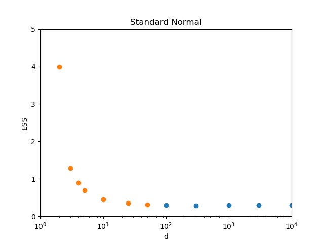
With some \(\epsilon\) stepsize in time, this is the improved inverse transform sampling¹, where a random number generator was replaced by a low-discrepancy sequence² generator, namely the additive recurrence. As such, it is very efficient and has \(ESS > 1\). This property persists in dimensions \(d = 2\) and \(d = 3\) as is shown in Figure 1 with the standard Gaussian target in various dimensions.

Derivation of MCLMC from the isokinetic method¶

As it turns out, one can derive the MCLMC ODE in a number of ways. One is to start by assuming the constraint that the norm of \(p\) is constant with time.

This was first done in the Molecular Dynamics community, under the name of the isokinetic method. (The authors of MCLMC became aware of this connection sometime after their original papers).

The idea is simply that we take Hamiltonian dynamics (with the potential energy \(S\) being the log likelihood of the target distribution as usual, and \(M=1\)) and add a constraint that \(\frac{d}{dt}(p^Tp)=0\) (by a Lagrange multiplier in the normal fashion):

\[ \frac{d}{dt}\begin{bmatrix} q \\ p \end{bmatrix} = \begin{bmatrix} p \\ -\nabla S(x) - \xi p \end{bmatrix} \]

Then the constraint implies that \(0 = p^T\dot p=p^T(-\nabla S(x) - \xi p)\) so that \(\xi = -p^T(\nabla S(x))(p^Tp)^{-1}\). Putting this back into the equation:

\[ \frac{d}{dt}\begin{bmatrix} q \\ p \end{bmatrix} = \begin{bmatrix} p \\ -\nabla S(x) +p^T(\nabla S(q))(p^Tp)^{-1}p \end{bmatrix}\]

\[ = \begin{bmatrix} p \\ (I - p(p^T(p^Tp)^{-1})) (-\nabla S(q)) \end{bmatrix}\]

\[ = \begin{bmatrix} p \\ (I - \mathcal{P}(p)) (-\nabla S(q)) \end{bmatrix} \\ \]

where \(\mathcal{P}\) is the projection operator onto the span of \(p\) (note its idempotency).

We can derive the stationary distribution (see the references) from the ansatz \(\rho(p,q) = e^{-w(p,q)}f(p^Tp)\), which after use of the continuity equation and some algebra gives:

\[ \rho(p,q) \propto e^{-\frac{(d-1)S(q)}{||p||^2}}\delta(||p|| - ||p_0||) \]

From here, we recover the MCLMC dynamics as given in the MCLMC paper by setting the initial \(||p_0||\) to \(1\). Further, we rescale \(S \mapsto S/(d-1)\).